transformers/docs/source/en/perf_train_gpu_one.mdx

<!--Copyright 2022 The HuggingFace Team. All rights reserved.

Licensed under the Apache License, Version 2.0 (the "License"); you may not use this file except in compliance with
the License. You may obtain a copy of the License at

http://www.apache.org/licenses/LICENSE-2.0

Unless required by applicable law or agreed to in writing, software distributed under the License is distributed on
an "AS IS" BASIS, WITHOUT WARRANTIES OR CONDITIONS OF ANY KIND, either express or implied. See the License for the
-->

# Efficient Training on a Single GPU

This guide focuses on training large models efficiently on a single GPU. These approaches are still valid if you have access to a machine with multiple GPUs but you will also have access to additional methods outlined in the [multi-GPU section](perf_train_gpu_many).

In this section we have a look at a few tricks to reduce the memory footprint and speed up training for large models and how they are integrated in the [`Trainer`] and [🤗 Accelerate](https://huggingface.co/docs/accelerate/). Each method can improve speed or memory usage which is summarized in the table below:

|Method|Speed|Memory|
|:-----|:----|:-----|
| Gradient accumulation | No | Yes |
| Gradient checkpointing | No| Yes |
| Mixed precision training | Yes | (No) |
| Batch size | Yes | Yes |
| Optimizer choice | Yes | Yes |
| DataLoader | Yes | No |
| DeepSpeed Zero | No | Yes |

A bracket means that it might not be strictly the case but is usually either not a main concern or negligible. Before we start make sure you have installed the following libraries:

```bash
pip install transformers datasets accelerate nvidia-ml-py3
```

The `nvidia-ml-py3` library allows us to monitor the memory usage of the models from within Python. You might be familiar with the `nvidia-smi` command in the terminal - this library allows to access the same information in Python directly.

Then we create some dummy data. We create random token IDs between 100 and 30000 and binary labels for a classifier. In total we get 512 sequences each with length 512 and store them in a [`~datasets.Dataset`] with PyTorch format.


```py
import numpy as np
from datasets import Dataset


seq_len, dataset_size = 512, 512
dummy_data = {
    "input_ids": np.random.randint(100, 30000, (dataset_size, seq_len)),
    "labels": np.random.randint(0, 1, (dataset_size)),
}
ds = Dataset.from_dict(dummy_data)
ds.set_format("pt")
```

We want to print some summary statistics for the GPU utilization and the training run with the [`Trainer`]. We setup a two helper functions to do just that:

```py
from pynvml import *


def print_gpu_utilization():
    nvmlInit()
    handle = nvmlDeviceGetHandleByIndex(0)
    info = nvmlDeviceGetMemoryInfo(handle)
    print(f"GPU memory occupied: {info.used//1024**2} MB.")


def print_summary(result):
    print(f"Time: {result.metrics['train_runtime']:.2f}")
    print(f"Samples/second: {result.metrics['train_samples_per_second']:.2f}")
    print_gpu_utilization()
```

Let's verify that we start with a free GPU memory:

```py
>>> print_gpu_utilization()
GPU memory occupied: 0 MB.
```

That looks good: the GPU memory is not occupied as we would expect before we load any models. If that's not the case on your machine make sure to stop all processes that are using GPU memory. However, not all free GPU memory can be used by the user. When a model is loaded to the GPU also the kernels are loaded which can take up 1-2GB of memory. To see how much it is we load a tiny tensor into the GPU which triggers the kernels to be loaded as well.

```py
>>> import torch


>>> torch.ones((1, 1)).to("cuda")
>>> print_gpu_utilization()
GPU memory occupied: 1343 MB.
```

We see that the kernels alone take up 1.3GB of GPU memory. Now let's see how much space the model uses.

## Load Model

First, we load the `bert-large-uncased` model. We load the model weights directly to the GPU so that we can check how much space just weights use.


```py
>>> from transformers import AutoModelForSequenceClassification


>>> model = AutoModelForSequenceClassification.from_pretrained("bert-large-uncased").to("cuda")
>>> print_gpu_utilization()
GPU memory occupied: 2631 MB.
```

We can see that the model weights alone take up 1.3 GB of the GPU memory. The exact number depends on the specific GPU you are using. Note that on newer GPUs a model can sometimes take up more space since the weights are loaded in an optimized fashion that speeds up the usage of the model. Now we can also quickly check if we get the same result as with `nvidia-smi` CLI:


```bash
nvidia-smi
```

```bash
Tue Jan 11 08:58:05 2022
+-----------------------------------------------------------------------------+
| NVIDIA-SMI 460.91.03    Driver Version: 460.91.03    CUDA Version: 11.2     |
|-------------------------------+----------------------+----------------------+
| GPU  Name        Persistence-M| Bus-Id        Disp.A | Volatile Uncorr. ECC |
| Fan  Temp  Perf  Pwr:Usage/Cap|         Memory-Usage | GPU-Util  Compute M. |
|                               |                      |               MIG M. |
|===============================+======================+======================|
|   0  Tesla V100-SXM2...  On   | 00000000:00:04.0 Off |                    0 |
| N/A   37C    P0    39W / 300W |   2631MiB / 16160MiB |      0%      Default |
|                               |                      |                  N/A |
+-------------------------------+----------------------+----------------------+

+-----------------------------------------------------------------------------+
| Processes:                                                                  |
|  GPU   GI   CI        PID   Type   Process name                  GPU Memory |
|        ID   ID                                                   Usage      |
|=============================================================================|
|    0   N/A  N/A      3721      C   ...nvs/codeparrot/bin/python     2629MiB |
+-----------------------------------------------------------------------------+
```

We get the same number as before and you can also see that we are using a V100 GPU with 16GB of memory. So now we can start training the model and see how the GPU memory consumption changes. First, we set up a few standard training arguments that we will use across all our experiments:

```py
default_args = {
    "output_dir": "tmp",
    "evaluation_strategy": "steps",
    "num_train_epochs": 1,
    "log_level": "error",
    "report_to": "none",
}
```

<Tip>

 Note: In order to properly clear the memory after experiments we need restart the Python kernel between experiments. Run all steps above and then just one of the experiments below.

</Tip>

## Vanilla Training

As a first experiment we will use the [`Trainer`] and train the model without any further modifications and a batch size of 4:

```py
from transformers import TrainingArguments, Trainer, logging

logging.set_verbosity_error()


training_args = TrainingArguments(per_device_train_batch_size=4, **default_args)
trainer = Trainer(model=model, args=training_args, train_dataset=ds)
result = trainer.train()
print_summary(result)
```

```
Time: 57.82
Samples/second: 8.86
GPU memory occupied: 14949 MB.
```

We see that already a relatively small batch size almost fills up our GPU's entire memory. However, a larger batch size can often result in faster model convergence or better end performance. So ideally we want to tune the batch size to our model's needs and not to the GPU limitations. What's interesting is that we use much more memory than the size of the model. To understand a bit better why this is the case let's have look at a model's operations and memory needs.

## Anatomy of Model's Operations

Transformers architecture includes 3 main groups of operations grouped below by compute-intensity.

1. **Tensor Contractions**

    Linear layers and components of Multi-Head Attention all do batched **matrix-matrix multiplications**. These operations are the most compute-intensive part of training a transformer.

2. **Statistical Normalizations**

    Softmax and layer normalization are less compute-intensive than tensor contractions, and involve one or more **reduction operations**, the result of which is then applied via a map.

3. **Element-wise Operators**

    These are the remaining operators: **biases, dropout, activations, and residual connections**. These are the least compute-intensive operations.

This knowledge can be helpful to know when analyzing performance bottlenecks.

This summary is derived from [Data Movement Is All You Need: A Case Study on Optimizing Transformers 2020](https://arxiv.org/abs/2007.00072)


## Anatomy of Model's Memory
We've seen that training the model uses much more memory than just putting the model on the GPU. This is because there are many components during training that use GPU memory. The components on GPU memory are the following:
1. model weights
2. optimizer states
3. gradients
4. forward activations saved for gradient computation
5. temporary buffers
6. functionality-specific memory

A typical model trained in mixed precision with AdamW requires 18 bytes per model parameter plus activation memory. For inference there are no optimizer states and gradients, so we can subtract those. And thus we end up with 6 bytes per model parameter for mixed precision inference, plus activation memory.

Let's look at the details.

**Model Weights:**

- 4 bytes * number of parameters for fp32 training
- 6 bytes * number of parameters for mixed precision training (maintains a model in fp32 and one in fp16 in memory)

**Optimizer States:**

- 8 bytes * number of parameters for normal AdamW (maintains 2 states)
- 2 bytes * number of parameters for 8-bit AdamW optimizers like [bitsandbytes](https://github.com/TimDettmers/bitsandbytes)
- 4 bytes * number of parameters for optimizers like SGD with momentum (maintains only 1 state)

**Gradients**

- 4 bytes * number of parameters for either fp32 or mixed precision training (gradients are always kept in fp32)

**Forward Activations**

- size depends on many factors, the key ones being sequence length, hidden size and batch size.

There are the input and output that are being passed and returned by the forward and the backward functions and the forward activations saved for gradient computation.

**Temporary Memory**

Additionally there are all kinds of temporary variables which get released once the calculation is done, but in the moment these could require additional memory and could push to OOM. Therefore when coding it's crucial to think strategically about such temporary variables and sometimes to explicitly free those as soon as they are no longer needed.

**Functionality-specific memory**

Then your software could have special memory needs. For example, when generating text using beam search, the software needs to maintain multiple copies of inputs and outputs.

**`forward` vs `backward` Execution Speed**

For convolutions and linear layers there are 2x flops in the backward compared to the forward, which generally translates into ~2x slower (sometimes more, because sizes in the backward tend to be more awkward). Activations are usually bandwidth-limited, and it’s typical for an activation to have to read more data in the backward than in the forward (e.g. activation forward reads once, writes once, activation backward reads twice, gradOutput and output of the forward, and writes once, gradInput).

So there are potentially a few places where we could save GPU memory or speed up operations. Let's start with a simple optimization: choosing the right batch size.

## Batch sizes

One gets the most efficient performance when batch sizes and input/output neuron counts are divisible by a certain number, which typically starts at 8, but can be much higher as well. That number varies a lot depending on the specific hardware being used and the dtype of the model.

For example for fully connected layers (which correspond to GEMMs), NVIDIA provides recommendations for [input/output neuron counts](
https://docs.nvidia.com/deeplearning/performance/dl-performance-fully-connected/index.html#input-features) and [batch size](https://docs.nvidia.com/deeplearning/performance/dl-performance-fully-connected/index.html#batch-size).

[Tensor Core Requirements](https://docs.nvidia.com/deeplearning/performance/dl-performance-matrix-multiplication/index.html#requirements-tc) define the multiplier based on the dtype and the hardware. For example, for fp16 a multiple of 8 is recommended, but on A100 it's 64!

For parameters that are small, there is also [Dimension Quantization Effects](https://docs.nvidia.com/deeplearning/performance/dl-performance-matrix-multiplication/index.html#dim-quantization) to consider, this is where tiling happens and the right multiplier can have a significant speedup.

## Gradient Accumulation

The idea behind gradient accumulation is to instead of calculating the gradients for the whole batch at once to do it in smaller steps. The way we do that is to calculate the gradients iteratively in smaller batches by doing a forward and backward pass through the model and accumulating the gradients in the process. When enough gradients are accumulated we run the model's optimization step. This way we can easily increase the overall batch size to numbers that would never fit into the GPU's memory. In turn, however, the added forward and backward passes can slow down the training a bit.

We can use gradient accumulation in the [`Trainer`] by simply adding the `gradient_accumulation_steps` argument to [`TrainingArguments`]. Let's see how it impacts the models memory footprint:

```py
training_args = TrainingArguments(per_device_train_batch_size=1, gradient_accumulation_steps=4, **default_args)

trainer = Trainer(model=model, args=training_args, train_dataset=ds)
result = trainer.train()
print_summary(result)
```

```
Time: 66.03
Samples/second: 7.75
GPU memory occupied: 8681 MB.
```

We can see that the memory footprint was dramatically reduced at the cost of being only slightly slower than the vanilla run. Of course, this would change as you increase the number of accumulation steps. In general you would want to max out the GPU usage as much as possible. So in our case, the batch_size of 4 was already pretty close to the GPU's limit. If we wanted to train with a batch size of 64 we should not use `per_device_train_batch_size=1` and `gradient_accumulation_steps=64` but instead `per_device_train_batch_size=4` and `gradient_accumulation_steps=16` which has the same effective batch size while making better use of the available GPU resources.

For more details see the benchmarks for [RTX-3090](https://github.com/huggingface/transformers/issues/14608#issuecomment-1004392537)
and [A100](https://github.com/huggingface/transformers/issues/15026#issuecomment-1005033957).

Next we have a look at another trick to save a little bit more GPU memory called gradient checkpointing.

## Gradient Checkpointing

Even when we set the batch size to 1 and use gradient accumulation we can still run out of memory when working with large models. In order to compute the gradients during the backward pass all activations from the forward pass are normally saved. This can create a big memory overhead. Alternatively, one could forget all activations during the forward pass and recompute them on demand during the backward pass. This would however add a significant computational overhead and slow down training.

Gradient checkpointing strikes a compromise between the two approaches and saves strategically selected activations throughout the computational graph so only a fraction of the activations need to be re-computed for the gradients. See [this great article](https://medium.com/tensorflow/fitting-larger-networks-into-memory-583e3c758ff9) explaining the ideas behind gradient checkpointing.

To enable gradient checkpointing in the [`Trainer`] we only need to pass it as a flag to the [`TrainingArguments`]. Everything else is handled under the hood:

```py
training_args = TrainingArguments(
    per_device_train_batch_size=1, gradient_accumulation_steps=4, gradient_checkpointing=True, **default_args
)

trainer = Trainer(model=model, args=training_args, train_dataset=ds)
result = trainer.train()
print_summary(result)
```

```
Time: 85.47
Samples/second: 5.99
GPU memory occupied: 6775 MB.
```

We can see that this saved some more memory but at the same time training became a bit slower. A general rule of thumb is that gradient checkpointing slows down training by about 20%. Let's have a look at another method with which we can regain some speed: mixed precision training.


## Floating Data Types

The idea of mixed precision training is that not all variables need to be stored in full (32-bit) floating point precision. If we can reduce the precision the variables and their computations are faster. Here are the commonly used floating point data types choice of which impacts both memory usage and throughput:

- fp32 (`float32`)
- fp16 (`float16`)
- bf16 (`bfloat16`)
- tf32 (CUDA internal data type)

Here is a diagram that shows how these data types correlate to each other.

![data types](https://huggingface.co/datasets/huggingface/documentation-images/resolve/main/tf32-bf16-fp16-fp32.png)
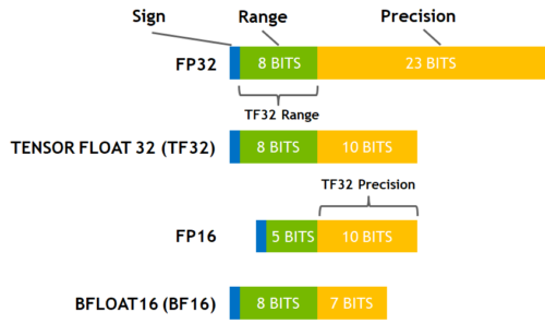
(source: [NVIDIA Blog](https://developer.nvidia.com/blog/accelerating-ai-training-with-tf32-tensor-cores/))

While fp16 and fp32 have been around for quite some time, bf16 and tf32 are only available on the Ampere architecture GPUS and TPUs support bf16 as well. Let's start with the most commonly used method which is FP16 training/


### FP16 Training

The idea of mixed precision training is that not all variables need to be stored in full (32-bit) floating point precision. If we can reduce the precision the variales and their computations are faster. The main advantage comes from saving the activations in half (16-bit) precision. Although the gradients are also computed in half precision they are converted back to full precision for the optimization step so no memory is saved here. Since the model is present on the GPU in both 16-bit and 32-bit precision this can use more GPU memory (1.5x the original model is on the GPU), especially for small batch sizes. Since some computations are performed in full and some in half precision this approach is also called mixed precision training. Enabling mixed precision training is also just a matter of setting the `fp16` flag to `True`:

```py
training_args = TrainingArguments(per_device_train_batch_size=4, fp16=True, **default_args)

trainer = Trainer(model=model, args=training_args, train_dataset=ds)
result = trainer.train()
print_summary(result)
```

```
Time: 27.46
Samples/second: 18.64
GPU memory occupied: 13939 MB.
```

We can see that this is almost twice as fast as the vanilla training. Let's add it to the mix of the previous methods:


```py
training_args = TrainingArguments(
    per_device_train_batch_size=1,
    gradient_accumulation_steps=4,
    gradient_checkpointing=True,
    fp16=True,
    **default_args,
)

trainer = Trainer(model=model, args=training_args, train_dataset=ds)
result = trainer.train()
print_summary(result)
```

```
Time: 50.76
Samples/second: 10.09
GPU memory occupied: 7275 MB.
```

We can see that with these tweaks we use about half the GPU memory as at the beginning while also being slightly faster.

### BF16
If you have access to a Ampere or newer hardware you can use bf16 for your training and evaluation. While bf16 has a worse precision than fp16, it has a much much bigger dynamic range. Therefore, if in the past you were experiencing overflow issues while training the model, bf16 will prevent this from happening most of the time. Remember that in fp16 the biggest number you can have is `65535` and any number above that will overflow. A bf16 number can be as large as `3.39e+38` (!) which is about the same as fp32 - because both have 8-bits used for the numerical range.

You can enable BF16 in the 🤗 Trainer with:

```python
TrainingArguments(bf16=True)
```

### TF32
The Ampere hardware uses a magical data type called tf32. It has the same numerical range as fp32 (8-bits), but instead of 23 bits precision it has only 10 bits (same as fp16) and uses only 19 bits in total.

It's magical in the sense that you can use the normal fp32 training and/or inference code and by enabling tf32 support you can get up to 3x throughput improvement. All you need to do is to add this to your code:

```
import torch
torch.backends.cuda.matmul.allow_tf32 = True
```

When this is done CUDA will automatically switch to using tf32 instead of fp32 where it's possible. This, of course, assumes that the used GPU is from the Ampere series.

Like all cases with reduced precision this may or may not be satisfactory for your needs, so you have to experiment and see. According to [NVIDIA research](https://developer.nvidia.com/blog/accelerating-ai-training-with-tf32-tensor-cores/) the majority of machine learning training shouldn't be impacted and showed the same perplexity and convergence as the fp32 training.

If you're already using fp16 or bf16 mixed precision it may help with the throughput as well.

You can enable this mode in the 🤗 Trainer with:
```python
TrainingArguments(tf32=True)
```
By default the PyTorch default is used.

Note: tf32 mode is internal to CUDA and can't be accessed directly via `tensor.to(dtype=torch.tf32)` as `torch.tf32` doesn't exist.

Note: you need `torch>=1.7` to enjoy this feature.

You can also see a variety of benchmarks on tf32 vs other precisions:
[RTX-3090](https://github.com/huggingface/transformers/issues/14608#issuecomment-1004390803) and
[A100](https://github.com/huggingface/transformers/issues/15026#issuecomment-1004543189).

We've now seen how we can change the floating types to increase throughput, but we are not done, yet! There is another area where we can save GPU memory: the optimizer.

## Optimizer

The most common optimizer used to train transformer model is Adam or AdamW (Adam with weight decay). Adam achieves good convergence by storing the rolling average of the previous gradients which, however, adds an additional memory footprint of the order of the number of model parameters. One remedy to this is to use an alternative optimizer such as Adafactor, which works well for some models but often it has instability issues.

HF Trainer integrates a variety of optimisers that can be used out of box. To activate the desired optimizer simply pass the `--optim` flag to the command line.

To see which optimizers are currently supported:

```bash
$ python examples/pytorch/translation/run_translation.py -h | grep "\-optim"
         [--optim {adamw_hf,adamw_torch,adamw_torch_xla,adamw_apex_fused,adafactor}]
```

For example, if you have [NVIDIA/apex](https://github.com/NVIDIA/apex) installed `--optim adamw_apex_fused` will give you the fastest training experience among all supported AdamW optimizers.

On the other hand [8bit BNB optimizer](https://github.com/TimDettmers/bitsandbytes) can save 3/4 of memory normally used by a typical AdamW optimizer if it is configured to quantize all optimizer states, but in some situations only some optimizer states are quintized and then more memory is used.

Let's get a feel for the numbers and use for example use a 3B-parameter model, like `t5-3b`. Note that since a Gigabyte correpsonds to a billion bytes we can simply multiply the parameters (in billions) with the number of necessary bytes per parameter to get Gigabytes of GPU memory usage:

- A standard AdamW uses 8 bytes for each parameter, here the optimizer will need (`8*3`) 24GB of GPU memory.
- Adafactor uses slightly more than 4 bytes, so (`4*3`) 12GB and then some extra.
- 8bit BNB quantized optimizer will use only (`2*3`) 6GB if all optimizer states are quantized.

Let's have a look at Adafactor first.

### Adafactor

Instead of keeping the rolling average for each element in the weight matrices Adafactor only stores aggregated information (row- and column-wise sums of the rolling averages) which reduces the footprint considerably. One downside of Adafactor is that in some instances convergence can be slower than Adam's so some experimentation is advised here. We can use Adafactor simply by setting `optim="adafactor"`:


```py
training_args = TrainingArguments(per_device_train_batch_size=4, optim="adafactor", **default_args)

trainer = Trainer(model=model, args=training_args, train_dataset=ds)
result = trainer.train()
print_summary(result)
```

```
Time: 64.31
Samples/second: 7.96
GPU memory occupied: 12295 MB.
```

We can see that this saves a few more GB on the GPU. Let's see how it looks when we add it to the other methods we introduced earlier:


```py
training_args = TrainingArguments(
    per_device_train_batch_size=1,
    gradient_accumulation_steps=4,
    gradient_checkpointing=True,
    fp16=True,
    optim="adafactor",
    **default_args,
)

trainer = Trainer(model=model, args=training_args, train_dataset=ds)
result = trainer.train()
print_summary(result)
```

```
Time: 56.54
Samples/second: 9.06
GPU memory occupied: 4847 MB.
```

We went from 15 GB memory usage to 5 GB - a 3x improvement while maintaining the throughput! However, as mentioned before, the convergence of Adafactor can be worse than Adam. There is an alternative to Adafactor called 8-bit Adam that takes a slightly different approach.

### 8-bit Adam

Instead of aggregating optimizer states like Adafactor, 8-bit Adam keeps the full state and quantizes it. Quantization means that it stores the state with lower precision and dequantizes it only for the optimization. This is similar to the idea behind FP16 training where using variables with lower precision saves memory.

In contrast to the previous approaches is this one not integrated into the [`Trainer`] as a simple flag. We need to install the 8-bit optimizer and then pass it as a custom optimizer to the [`Trainer`]. Follow the installation guide in the Github [repo](https://github.com/TimDettmers/bitsandbytes) to install the `bitsandbytes` library that implements the 8-bit Adam optimizer.

Once installed, we just need to initialize the the optimizer. Although this looks like a considerable amount of work it actually just involves two steps: first we need to group the model's parameters into two groups where to one group we apply weight decay and to the other we don't. Usually, biases and layer norm parameters are not weight decayed. Then in a second step we just do some argument housekeeping to use the same parameters as the previously used AdamW optimizer.

<Tip>
Note that in order to use the 8-bit optimizer with an existing pretrained model a change to the embedding layer is needed.
Read [this issue](https://github.com/huggingface/transformers/issues/14819) for more information.
</Tip>

```py
import bitsandbytes as bnb
from torch import nn
from transformers.trainer_pt_utils import get_parameter_names

training_args = TrainingArguments(per_device_train_batch_size=4, **default_args)

decay_parameters = get_parameter_names(model, [nn.LayerNorm])
decay_parameters = [name for name in decay_parameters if "bias" not in name]
optimizer_grouped_parameters = [
    {
        "params": [p for n, p in model.named_parameters() if n in decay_parameters],
        "weight_decay": training_args.weight_decay,
    },
    {
        "params": [p for n, p in model.named_parameters() if n not in decay_parameters],
        "weight_decay": 0.0,
    },
]

optimizer_kwargs = {
    "betas": (training_args.adam_beta1, training_args.adam_beta2),
    "eps": training_args.adam_epsilon,
}
optimizer_kwargs["lr"] = training_args.learning_rate
adam_bnb_optim = bnb.optim.Adam8bit(
    optimizer_grouped_parameters,
    betas=(training_args.adam_beta1, training_args.adam_beta2),
    eps=training_args.adam_epsilon,
    lr=training_args.learning_rate,
)
```

We can now pass the custom optimizer as an argument to the `Trainer`:
```py
trainer = Trainer(model=model, args=training_args, train_dataset=ds, optimizers=(adam_bnb_optim, None))
result = trainer.train()
print_summary(result)
```

```
Time: 55.95
Samples/second: 9.15
GPU memory occupied: 13085 MB.
```

We can see that we get a similar memory improvement as with Adafactor while keeping the full rolling average of the gradients. Let's repeat the experiment with the full settings:

```py
training_args = TrainingArguments(
    per_device_train_batch_size=1,
    gradient_accumulation_steps=4,
    gradient_checkpointing=True,
    fp16=True,
    **default_args,
)

trainer = Trainer(model=model, args=training_args, train_dataset=ds, optimizers=(adam_bnb_optim, None))
result = trainer.train()
print_summary(result)
```

```
Time: 49.46
Samples/second: 10.35
GPU memory occupied: 5363 MB.
```

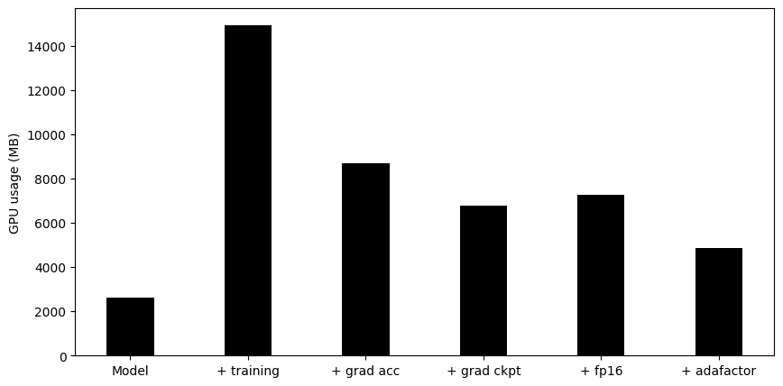
Again, we get about a 3x memory improvement and even slightly higher throughput as using Adafactor. So we have seen how we can optimize the memory footprint of large models. The following plot summarizes all our experiments:

![png](https://huggingface.co/datasets/lvwerra/repo-images/raw/main/gpu-memory-savings.png)

### `_multi_tensor`
pytorch-nightly introduced `torch.optim._multi_tensor` which should significantly speed up the optimizers for situations with lots of small feature tensors. It should eventually become the default, but if you want to experiment with it sooner and don't mind using the bleed-edge, see: https://github.com/huggingface/transformers/issues/9965


## Using 🤗 Accelerate

So far we have used the [`Trainer`] to run the experiments but a more flexible alternative to that approach is to use 🤗 Accelerate. With 🤗 Accelerate you have full control over the training loop and can essentially write the loop in pure PyTorch with some minor modifications. In turn it allows you to easily scale across different infrastructures such as CPUs, GPUs, TPUs, or distributed multi-GPU setups without changing any code. Let's see what it takes to implement all of the above tweaks in 🤗 Accelerate. We can still use the [`TrainingArguments`] to wrap the training settings:


```py
training_args = TrainingArguments(
    per_device_train_batch_size=1,
    gradient_accumulation_steps=4,
    gradient_checkpointing=True,
    fp16=True,
    **default_args,
)
```

The full example training loop with 🤗 Accelerate is only a handful of lines of code long:


```py
from accelerate import Accelerator
from torch.utils.data.dataloader import DataLoader

dataloader = DataLoader(ds, batch_size=training_args.per_device_train_batch_size)

if training_args.gradient_checkpointing:
    model.gradient_checkpointing_enable()

accelerator = Accelerator(fp16=training_args.fp16)
model, optimizer, dataloader = accelerator.prepare(model, adam_bnb_optim, dataloader)

model.train()
for step, batch in enumerate(dataloader, start=1):
    loss = model(**batch).loss
    loss = loss / training_args.gradient_accumulation_steps
    accelerator.backward(loss)
    if step % training_args.gradient_accumulation_steps == 0:
        optimizer.step()
        optimizer.zero_grad()
```

First we wrap the dataset in a [`DataLoader`](https://pytorch.org/docs/stable/data.html#torch.utils.data.DataLoader). Then we can enable gradient checkpointing by calling the model's [`~PreTrainedModel.gradient_checkpointing_enable`] method. When we initialize the [`Accelerator`](https://huggingface.co/docs/accelerate/package_reference/accelerator#accelerate.Accelerator) we can specify if we want to use mixed precision training and it will take care of it for us in the [`prepare`] call. During the [`prepare`](https://huggingface.co/docs/accelerate/package_reference/accelerator#accelerate.Accelerator.prepare) call the dataloader will also be distributed across workers should we use multiple GPUs. We use the same 8-bit optimizer from the earlier experiments.

Finally, we can write the main training loop. Note that the `backward` call is handled by 🤗 Accelerate. We can also see how gradient accumulation works: we normalize the loss so we get the average at the end of accumulation and once we have enough steps we run the optimization. Now the question is: does this use the same amount of memory as the previous steps? Let's check:


```py
>>> print_gpu_utilization()
GPU memory occupied: 5363 MB.
```

Indeed it does. Implementing these optimization techniques with 🤗 Accelerate only takes a handful of lines of code and comes with the benefit of more flexiblity in the training loop. For a full documentation of all features have a look at the [Accelerate documentation](https://huggingface.co/docs/accelerate/index).

## DataLoader

One of the important requirements to reach great training speed is the ability to feed the GPU at the maximum speed it can handle. By default everything happens in the main process and it might not be able to read the data from disk fast enough, and thus create a bottleneck, leading to GPU under-utilization.

- `DataLoader(pin_memory=True, ...)` which ensures that the data gets preloaded into the pinned memory on CPU and typically leads to much faster transfers from CPU to GPU memory.
- `DataLoader(num_workers=4, ...)` - spawn several workers to pre-load data faster - during training watch the GPU utilization stats and if it's far from 100% experiment with raising the number of workers. Of course, the problem could be elsewhere so a very big number of workers won't necessarily lead to a better performance.

## DeepSpeed ZeRO

The in-depth details on how to use Deepspeed can be found [here](main_classes/deepspeed).

First, a quick decision tree:

1. Model fits onto a single GPU and you have enough space to fit a small batch size - you don't need to use Deepspeed as it'll only slow things down in this use case.
2. Model doesn't fit onto a single GPU or you can't fit a small batch - use DeepSpeed ZeRO + CPU Offload and for much larger models NVMe Offload.

Now if the decision tree suggested you use DeepSpeed first you need to [install it](main_classes/deepspeed#installation), then follow one of the following guides to create a configuration file and launch DeepSpeed.

Activation:

- HF Trainer-based examples: see this [guide](main_classes/deepspeed#deployment-with-one-gpu).
- Custom HF Trainer-based program: Same as above, but pass:

    ```python
    TrainingArguments(deepspeed="/path/to/ds_config.json")
    ```
- Deployment in Notebooks: see this [guide](main_classes/deepspeed#deployment-in-notebooks).

- Custom training loop: This is somewhat complex but you can study how this is implemented in [HF Trainer](
https://github.com/huggingface/transformers/blob/master/src/transformers/trainer.py) - simply search for `deepspeed` in the code.


## Choice of GPU
Sometimes, even when applying all the above tweaks the throughput on a given GPU might still not be good enough. One easy solution is to change the type of GPU. For example switching from let's say a K80 (which you typically get on Google Colab) to a fancier GPU such as the V100 or A100. Although they are more expensive they are usually more cost effective than cheaper GPUs due to their larger memory and faster architecture.

Now, let's take a step back and discuss what we should optimize for when scaling the training of large models.

## How to scale

When we train models there are a two aspects we want to optimize at the same time:

- Data throughput/training time
- Model performance

We have seen that each method changes the memory usage and throughput. In general we want to maximize the throughput (samples/second) to minimize the training cost. This is generally achieved by utilizing the GPU as much as possible and thus filling GPU memory to its limit. For example, as mentioned earlier, we only employ gradient accumulation when we want to use a batch size beyond the size of the GPU memory. If the desired batch size fits into memory then there is no reason to apply gradient accumulation which will only slow down training.

The second objective is model performance. Just because we can does not mean we should use a large batch size. As part of hyperparameter tuning you should determine which batch size yields the best result and then optimize the throughput accordingly.


## Efficient Software Prebuilds

PyTorch's [pip and conda builds](https://pytorch.org/get-started/locally/#start-locally) come prebuit with the cuda toolkit which is enough to run PyTorch, but it is insufficient if you need to build cuda extensions.

At times it may take an additional effort to pre-build some components, e.g., if you're using libraries like `apex` that don't come pre-compiled. In other situations figuring out how to install the right cuda toolkit system-wide can be complicated. To address these users' needs PyTorch and NVIDIA release a new version of NGC docker container which already comes with everything prebuilt and you just need to install your programs on it and it will run out of the box.

This approach is also useful if you want to tweak the pytorch source and/or make a new customized build.

To find the docker image version you want start [here](https://docs.nvidia.com/deeplearning/frameworks/pytorch-release-notes/), choose one of the latest monthly releases. Go into the release's notes for the desired release, check that the environment's components are matching your needs (including NVIDIA Driver requirements!) and then at the very top of that document go to the corresponding NGC page. If for some reason you get lost, here is [the index of all PyTorch NGC images](https://ngc.nvidia.com/catalog/containers/nvidia:pytorch).

Next follow the instructions to download and deploy the docker image.

## Sparsity

### Mixture of Experts

Quite a few of the recent papers reported a 4-5x training speedup and a faster inference by integrating
Mixture of Experts (MoE) into the Transformer models.

Since it has been discovered that more parameters lead to better performance, this technique allows to increase the number of parameters by an order of magnitude without increasing training costs.

In this approach every other FFN layer is replaced with a MoE Layer which consists of many experts, with a gated function that trains each expert in a balanced way depending on the input token's position in a sequence.

![MoE Transformer 2x block](https://huggingface.co/datasets/huggingface/documentation-images/resolve/main/perf-moe-transformer.png)

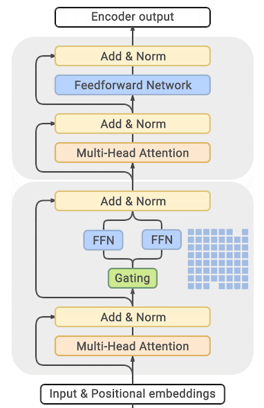
(source: [GLAM](https://ai.googleblog.com/2021/12/more-efficient-in-context-learning-with.html))

You can find exhaustive details and comparison tables in the papers listed at the end of this section.

The main drawback of this approach is that it requires staggering amounts of GPU memory - almost an order of magnitude larger than its dense equivalent. Various distillation and approaches are proposed to how to overcome the much higher memory requirements.

There is direct trade-off though, you can use just a few experts with a 2-3x smaller base model instead of dozens or hundreds experts leading to a 5x smaller model and thus increase the training speed moderately while increasing the memory requirements moderately as well.

Most related papers and implementations are built around Tensorflow/TPUs:

- [GShard: Scaling Giant Models with Conditional Computation and Automatic Sharding](https://arxiv.org/abs/2006.16668)
- [Switch Transformers: Scaling to Trillion Parameter Models with Simple and Efficient Sparsity](https://arxiv.org/abs/2101.03961)
- [GLaM: Generalist Language Model (GLaM)](https://ai.googleblog.com/2021/12/more-efficient-in-context-learning-with.html)

And for Pytorch DeepSpeed has built one as well: [DeepSpeed-MoE: Advancing Mixture-of-Experts Inference and Training to Power Next-Generation AI Scale](https://arxiv.org/abs/2201.05596), [Mixture of Experts](https://www.deepspeed.ai/tutorials/mixture-of-experts/) - blog posts:  [1](https://www.microsoft.com/en-us/research/blog/deepspeed-powers-8x-larger-moe-model-training-with-high-performance/), [2](https://www.microsoft.com/en-us/research/publication/scalable-and-efficient-moe-training-for-multitask-multilingual-models/) and specific deployment with large transformer-based natural language generation models: [blog post](https://www.deepspeed.ai/news/2021/12/09/deepspeed-moe-nlg.html), [Megatron-Deepspeed branch](Thttps://github.com/microsoft/Megatron-DeepSpeed/tree/moe-training).


## Scaling beyond a single GPU

For some applications, such as pretraining large language models, applying all the approaches above might still not be fast enough. In this case you want to scale your experiment to several GPUs.

Another use case for training on many GPUs is if the model does not fit on a single GPU with all the mentioned tricks. There are still more methods we can apply although life starts to get a bit more complicated. This usually involves some form of pipeline or tensor parallelism where the model itself is distributed across several GPUs. One can also make use of DeepSpeed which implements some of these parallelism strategies along with some more optimization to reduce the memory footprint such as partitioning the optimizer states. You can read more about this in the ["Multi-GPU training" section](perf_train_gpu_many).

## Using torch.compile

PyTorch 2.0 introduces a new compile function, you can learn more about it [in their documentation](https://pytorch.org/get-started/pytorch-2.0/). It uses Python’s frame evaluation API to automatically create a graph from existing PyTorch programs. After capturing the graph, different backends can be deployed to lower the graph to an optimized engine. You can choose one option below for performance boost.

`torch.compile` has a growing list of backends, which can be found in [backends.py](https://github.com/pytorch/pytorch/blob/master/torch/_dynamo/optimizations/backends.py)
or `torchdynamo.list_backends()` each of which with its optional dependencies.

Some of the most commonly used backends are

**Debugging backends**:
* `dynamo.optimize("eager")` - Uses PyTorch to run the extracted GraphModule. This is quite useful in debugging TorchDynamo issues.
* `dynamo.optimize("aot_eager")` - Uses AotAutograd with no compiler, i.e, just using PyTorch eager for the AotAutograd's extracted forward and backward graphs. This is useful for debugging, and unlikely to give speedups.

**Training & inference backends**:
* `dynamo.optimize("inductor")` - Uses TorchInductor backend with AotAutograd and cudagraphs by leveraging codegened Triton kernels  [Read more](https://dev-discuss.pytorch.org/t/torchinductor-a-pytorch-native-compiler-with-define-by-run-ir-and-symbolic-shapes/747)
* `dynamo.optimize("nvfuser")` -  nvFuser with TorchScript. [Read more](https://dev-discuss.pytorch.org/t/tracing-with-primitives-update-1-nvfuser-and-its-primitives/593)
* `dynamo.optimize("aot_nvfuser")` -  nvFuser with AotAutograd. [Read more](https://dev-discuss.pytorch.org/t/tracing-with-primitives-update-1-nvfuser-and-its-primitives/593)
* `dynamo.optimize("aot_cudagraphs")` - cudagraphs with AotAutograd. [Read more](https://github.com/pytorch/torchdynamo/pull/757)

**Inference-only backend**s:
* `dynamo.optimize("ofi")` -  Uses Torchscript optimize_for_inference.  [Read more](https://pytorch.org/docs/stable/generated/torch.jit.optimize_for_inference.html)
* `dynamo.optimize("fx2trt")` -  Uses Nvidia TensorRT for inference optimizations.  [Read more](https://github.com/pytorch/TensorRT/blob/master/docsrc/tutorials/getting_started_with_fx_path.rst)
* `dynamo.optimize("onnxrt")` -  Uses ONNXRT for inference on CPU/GPU.  [Read more](https://onnxruntime.ai/)
* `dynamo.optimize("ipex")` -  Uses IPEX for inference on CPU.  [Read more](https://github.com/intel/intel-extension-for-pytorch)